Going to Production
Going to production checklist for AI applications.
This guide will help you to prepare your application for production. We'll provide actionable steps to help you scale your application, ensure that it is reliable, can handle the load, and provide optimal accuracy for your use case.
See our Engineering for Scale guide for more information about engineering at scale.
Do you need indexes?#
Sequential scans will result in significantly higher latencies and lower throughput, guaranteeing 100% accuracy and not being RAM bound.
There are a couple of cases where you might not need indexes:
- You have a small dataset and don't need to scale it.
- You are not expecting high amounts of vector search queries per second.
- You need to guarantee 100% accuracy.
You don't have to create indexes in these cases and can use sequential scans instead. This type of workload will not be RAM bound and will not require any additional resources but will result in higher latencies and lower throughput. Extra CPU cores may help to improve queries per second, but it will not help to improve latency.
On the other hand, if you need to scale your application, you will need to create indexes. This will result in lower latencies and higher throughput, but will require additional RAM to make use of Postgres Caching. Also, using indexes will result in lower accuracy, since you are replacing exact (KNN) search with approximate (ANN) search.
HNSW vs IVFFlat indexes#
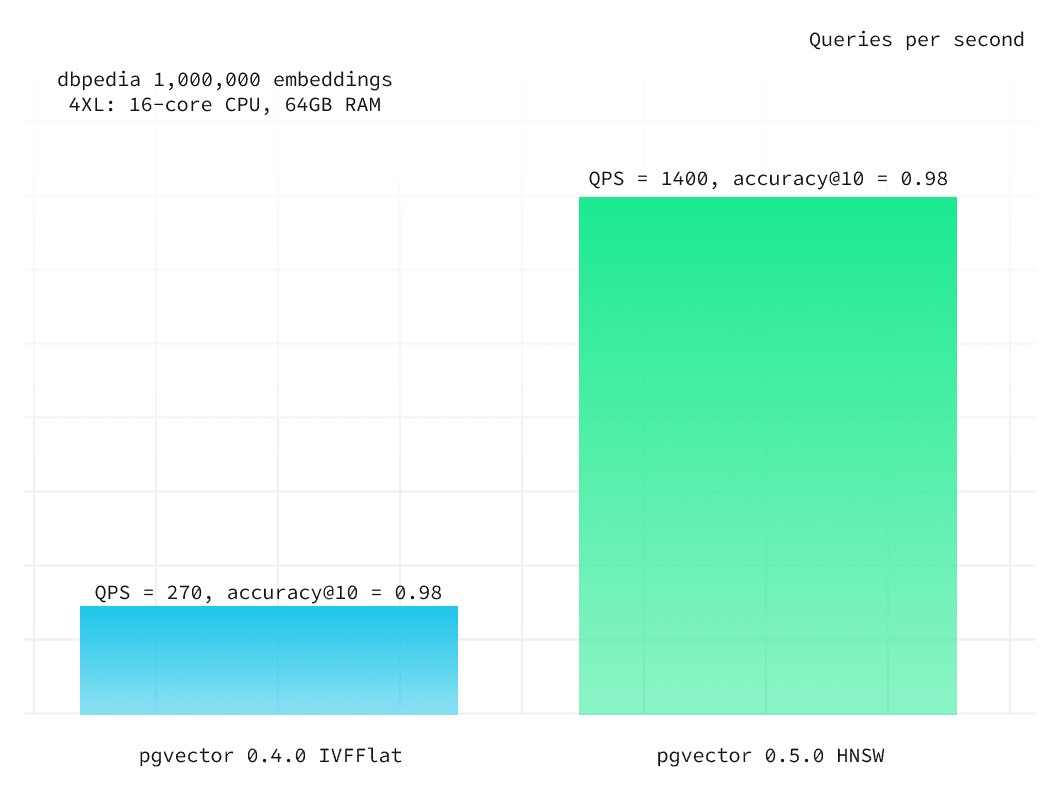
pgvector supports two types of indexes: HNSW and IVFFlat. We recommend using HNSW because of its performance and robustness against changing data.
HNSW, understanding ef_construction, ef_search, and m#
Index build parameters:
-
mis the number of bi-directional links created for every new element during construction. Highermis suitable for datasets with high dimensionality and/or high accuracy requirements. Reasonable values formare between 2 and 100. Range 12-48 is a good starting point for most use cases (16 is the default value). -
ef_constructionis the size of the dynamic list for the nearest neighbors (used during the construction algorithm). Higheref_constructionwill result in better index quality and higher accuracy, but it will also increase the time required to build the index.ef_constructionhas to be at least 2 *m(64 is the default value). At some point, increasingef_constructiondoes not improve the quality of the index. You can measure accuracy whenef_search=ef_construction: if accuracy is lower than 0.9, then there is room for improvement.
Search parameters:
ef_searchis the size of the dynamic list for the nearest neighbors (used during the search). Increasingef_searchwill result in better accuracy, but it will also increase the time required to execute a query (40 is the default value).

IVFFlat, understanding probes and lists#
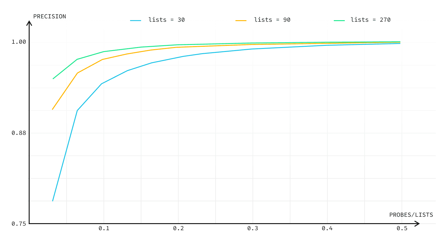
Indexes used for approximate vector similarity search in pgvector divides a dataset into partitions. The number of these partitions is defined by the lists constant. The probes controls how many lists are going to be searched during a query.
The values of lists and probes directly affect accuracy and queries per second (QPS).
- Higher
listsmeans an index will be built slower, but you can achieve better QPS and accuracy. - Higher
probesmeans that select queries will be slower, but you can achieve better accuracy. listsandprobesare not independent. Higherlistsmeans that you will have to use higherprobesto achieve the same accuracy.
You can find more examples of how lists and probes constants affect accuracy and QPS in pgvector 0.4.0 performance blogpost.
The chart below shows how the IVFFlat lists count affects accuracy and queries-per-second.
Performance tips when using indexes#
First, a few generic tips which you can pick and choose from:
- The Supabase managed platform will automatically optimize Postgres configs for you based on your compute add-on. But if you self-host, consider adjusting your Postgres config based on RAM & CPU cores. See example optimizations for more details.
- Prefer
inner-producttoL2orCosinedistances if your vectors are normalized (liketext-embedding-ada-002). If embeddings are not normalized,Cosinedistance should give the best results with an index. - Pre-warm your database. Implement the warm-up technique before transitioning to production or running benchmarks.
- Use pg_prewarm to load the index into RAM
select pg_prewarm('vecs.docs_vec_idx');. This will help to avoid cold cache issues. - Execute 10,000 to 50,000 "warm-up" queries before each benchmark or prod. This helps to use cache and buffers more efficiently.
- Use pg_prewarm to load the index into RAM
- Establish your workload. Fine-tune
mandef_constructionorlistsconstants for the pgvector index to accelerate your queries (at the expense of a slower build times). For instance, for benchmarks with 1,000,000 OpenAI embeddings, we setmandef_constructionto 32 and 80, and it resulted in 35% higher QPS than 24 and 56 values respectively. - Benchmark your own specific workloads. Doing this during cache warm-up helps gauge the best value for the index build parameters, balancing accuracy with queries per second (QPS).
Going into production#
- Decide if you are going to use indexes or not. You can skip the rest of this guide if you do not use indexes.
- Over-provision RAM during preparation. You can scale down in step
5, but it's better to start with a larger size to get the best results for RAM requirements. (We'd recommend at least 8XL if you're using Supabase.) - Upload your data to the database. If you use the
vecslibrary, it will automatically generate an index with default parameters. - Run a benchmark using randomly generated queries and observe the results. Again, you can use the
vecslibrary with theann-benchmarkstool. Do it with default values for index build parameters, you can later adjust them to get the best results. - Monitor the RAM usage, and save it as a note for yourself. You would likely want to use a compute add-on in the future that has the same amount of RAM that was used at the moment (both actual RAM usage and RAM used for cache and buffers).
- Scale down your compute add-on to the one that would have the same amount of RAM used at the moment.
- Repeat step 3 to load the data into RAM. You should see QPS increase on subsequent runs, and stop when it no longer increases.
- Run a benchmark using real queries and observe the results. You can use the
vecslibrary for that as well withann-benchmarkstool. Tweakef_searchfor HNSW orprobesfor IVFFlat until you see that both accuracy and QPS match your requirements. - If you want higher QPS you can increase
mandef_constructionfor HNSW orlistsfor IVFFlat parameters (consider switching from IVF to HNSW). You have to rebuild the index with a highermandef_constructionvalues and repeat steps 6-7 to find the best combination ofm,ef_constructionandef_searchconstants to achieve the best QPS and accuracy values. Higherm,ef_constructionmean that index will build slower, but you can achieve better QPS and accuracy. Higheref_searchmean that select queries will be slower, but you can achieve better accuracy.
Useful links#
Don't forget to check out the general Production Checklist to ensure your project is secure, performant, and will remain available for your users.
You can look at our Choosing Compute Add-on guide to get a basic understanding of how much compute you might need for your workload.
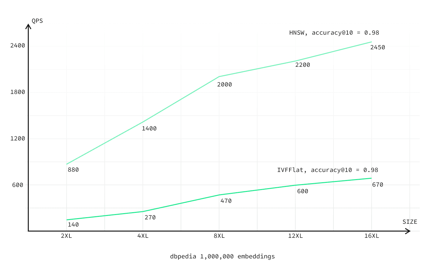
Or take a look at our pgvector 0.5.0 performance and pgvector 0.4.0 performance blog posts to see what pgvector is capable of and how the above technique can be used to achieve the best results.
The chart below plots requests-per-second against compute size.